Salt of the Sea Reading Level Rise

Suggested Citation:"2 Measured Global Ocean-Level Ascent." National Research Council. 2012. Sea-Level Rising for the Coasts of California, Oregon, and Washington: Past, Present, and Future. Washington, DC: The National Academies Press. doi: 10.17226/13389.

×

2

Measured Global Sea-Level Ascension

Rates of global bounding main-level rise over the past several millennia are inferred from geological and archeological (proxy) evidence. Modernistic rates are estimated using tide cuff measurements, which in some places appointment back to the 17th century, and satellite altimetry measurements of ocean-surface heights, which have been available for the past two decades. Gravity Recovery and Climate Experiment (GRACE) satellite measurements, start in 2002, offer a possible additional guess of global sea level.

Following a few 1000 years of relative stability, global ocean level began rising shortly after the beginning of the industrial era. The Intergovernmental Panel on Climate Change (IPCC) Fourth Assessment Report estimated that more modern rates of ocean-level rise began sometime betwixt the mid-19th and mid-20th centuries, based on geological and archeological observations and some of the longest tide gage records (Bindoff et al., 2007). Tide cuff measurements point that global mean ocean level rose 1.7 ± 0.5 mm twelvemonth^-1 over the 20th century and i.8 ± 0.5 mm yr^-1 from 1961 to 2003. Rates from satellite altimetry and tide gages were higher from 1993 to 2003—3.1 ± 0.7 mm yr^-1—only the IPCC was unable to determine whether the college charge per unit was due to decadal variability of the oceans or to an acceleration in body of water-level rise. This affiliate describes how sea level is measured and summarizes rates of body of water-level rise estimated since the IPCC Fourth Assessment Study was published.

PROXY MEASUREMENTS

Salt-marsh sediments, micro-atolls, and archaeological indicators are capable of capturing sub-meter-scale body of water-level changes during the by 2000 years (Box two.i). The near robust betoken in these proxy records is an acceleration from relatively low rates of sea-level change during the past two millennia (order 0.one mm yr^-1) to college mod rates of sea-level rise (2–3 mm year^-ane; e.g., Lambeck et al., 2004; Gehrels, 2010; Kemp et al., 2011). Both the magnitude and timing of the acceleration vary among reconstructions, likely considering of different assumptions almost the underlying geophysical processes and uncertainties in determining height and time from proxy records. Recent reconstructions place the onset of acceleration in sea-level ascension between 1840 and 1920 (Donnelly et al., 2004; Gehrels et al., 2006, 2008; Kemp et al., 2009, 2011). This late 19th or early on 20th century dispatch in sea-level rising is besides visible in the longest tide gage records of Brest (Wöppelmann et al., 2008), Amsterdam (Jevrejeva et al., 2008), Liverpool (Woodworth, 1999), Stockholm (Ekman, 1988), and San Francisco (Billow and Ruzmaikin, 2010).

TIDE GAGES

Tide gages measure the water level at the location of the gage (Box 2.two). Originally designed for navigational purposes, the outset gages began operating in the ports of Stockholm, Sweden, and Amsterdam, Holland, in the 17th century. There are at present more

Suggested Citation:"2 Measured Global Ocean-Level Ascension." National Research Council. 2012. Sea-Level Rise for the Coasts of California, Oregon, and Washington: By, Present, and Future. Washington, DC: The National Academies Press. doi: 10.17226/13389.

×

BOX 2.1
Inferring Sea Level from Proxy Measurements

Sea-level "proxies" are natural archives that record rates of sea-level ascension prior to the mid-19th century, when tide gage measurements became relatively common. Proxy indicators are generally calibrated confronting data from mod instruments and then used to reconstruct by sea levels. 3 types of proxy archives can be measured with sufficient precision to be compared with the instrumental record: salt-marsh sediments, micro-atolls, and archaeological observations. Stratigraphic sequences from common salt marshes tape changes in the frequency and duration of tidal inundation, and thus past sea levels. The recent discovery of correlations betwixt microfossils, such equally foraminifera, and tidal acme has significantly improved the precision of many sea-level reconstructions based on salt marshes (Horton and Edwards, 2006). Coral microatolls grow in a narrow range of sea levels. Growth at the upper surface of the coral potentially records fluctuations in relative body of water level (e.1000., Smithers and Woodroffe, 2001). Finally, some archaeological observations are relatable to sea level, including coastal h2o wells and Roman fish ponds (e.k., Lambeck et al., 2004).

Detailed proxy studies take non been done along the due west coast of the United states of america. An instance of the use of table salt-marsh sediments from N Carolina to approximate rates of sea-level rise is shown in the figure below. Analysis of sediment cores propose that the rate of body of water-level rise changed iii times: increasing betwixt 853 and 1076, decreasing between 1274 and 1476, then substantially increasing betwixt 1865 and 1892 (Kemp et al., 2011).

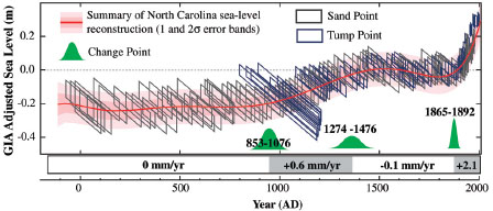
Figure Two k years of bounding main-level rise estimates from two Northward Carolina salt marshes (Sand Point and Tump Point). Errors in the data are represented by parallelograms; the correction for glacial isostatic aligning is larger at the old cease of the mistake box. The cerise line is the best fit to the body of water-level data. Green shapes indicate when significant changes occurred in the rate of sea-level rise. SOURCE: Kemp et al. (2011).

than 2,000 tide gages worldwide, most of which were established since 1950 (Jevrejeva et al., 2006).

By averaging the water levels measured at the cuff over a long flow of fourth dimension (daily, monthly), the outcome of daily tides is removed, leaving only the relative body of water level. This water level reflects not only the sea level, only also the effects of the weather, such as persistent wind systems and changes in atmospheric pressure; interannual to decadal climate variability; changes in oceanic currents; and vertical motions of the state on which the gage sits. These effects must be removed from the tide gage measurement to obtain the change in sea level caused past changes in ocean water volume or mass (encounter Appendix A).

The global mean sea level is adamant by spatially averaging all of the qualified tide gage records from around the world. Spatial averaging provides a means to avoid bias due to regional climate variations. Sampling bias due to the small number of tide gages, particularly earlier 1950, and their concentration in the Northern Hemisphere and forth coasts and islands is a major source of uncertainty in body of water-level modify estimates (Peltier and Tushingham, 1989; Church, 2001; Holgate and Woodworth, 2004). Long tide gage records (e.g., at least fifty–60 years) are usually used to boilerplate out decadal variability of the oceans' surface (Douglas, 1992).

The charge per unit of ocean-level modify is estimated by fitting a bend through the historical tide cuff readings. The bend could be a straight line or a higher social club polynomial over the whole length of the tape or shorter sections. More sophisticated data-dependent decompositions of the tide gage record also have been used (eastward.m., Peltier and Tushingham, 1989; Moore et al.,

Suggested Commendation:"2 Measured Global Body of water-Level Rise." National Research Council. 2012. Sea-Level Rise for the Coasts of California, Oregon, and Washington: By, Present, and Future. Washington, DC: The National Academies Press. doi: 10.17226/13389.

×

BOX two.ii
Tide Gage Measurements

Tide gages measure the peak of the h2o relative to a monitored geodetic benchmark on land (Effigy). Tide gages originally used a float to runway the water level inside a vertical tube. The bottom of the tube was closed except for a hole that permitted a pocket-size amount of h2o to enter the tube with fourth dimension, thus serving every bit a temporal filter. Slow changes in the sea surface acquired by tides or tempest surges accept sufficient time to fill the tube, while passing waves do not. Today, electronic sensors or bubbler gages have replaced tide gage floats.

Two organizations collect and preserve tide gage records from around the world: the Global Body of water Level Observing System, which has established a network of 290 tide gages worldwide; and the Permanent Service for Mean Body of water Level, which stores and disseminates the tidal records from more than than 2,000 stations around the world.

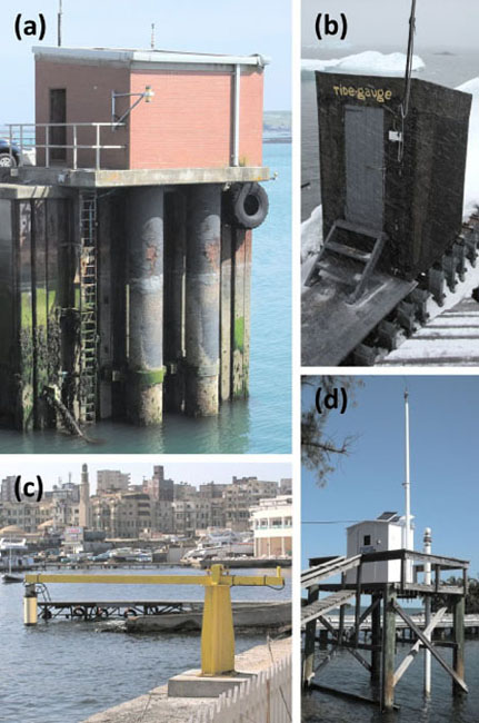
FIGURE Examples of tide gage stations. (a) A bladder and stilling-well gage at Holyhead, UK. SOURCE: Britain National Oceanography Heart. (b) A float gage at Vernadsky, Antarctica. SOURCE: British Antarctic Survey. (c) A radar tide gage at Alexandria, Arab republic of egypt. SOURCE: Courtesy of T. Aarup, Intergovernmental Oceanographic Commission. (d) An acoustic gage at Vaca Key, Florida. Acoustic gages at present course the majority of the U.Due south. sea-level network. SOURCE: National Oceanic and Atmospheric Administration.

Suggested Citation:"2 Measured Global Bounding main-Level Rise." National Research Quango. 2012. Sea-Level Rise for the Coasts of California, Oregon, and Washington: By, Nowadays, and Future. Washington, DC: The National Academies Press. doi: 10.17226/13389.

×

2005; Jevrejeva et al., 2006). Considering ocean level exhibits considerable interannual and decadal variability, the calculated rate of change depends on the length and start appointment of the record used. For example, Church building and White (2006) found that the global charge per unit of sea-level rising was i.7 ± 0.3 mm yr^-1 for the 20th century, 0.71 ± 0.4 mm yr^-1 for 1870–1935, and 1.84 ± 0.xix mm yr^-ane for 1936–2001. Their results are shown in Effigy 2.1, compared to other independent estimates of global sea-level rise from tide gages.

The time dependency of global ocean level can be seen in the assay of Church and White (2011), who calculated the body of water-level ascent using 16-twelvemonth moving windows of data, as shown in Effigy 2.ii (run into besides Box A.1 in Appendix A). In this example, the linear trend in global sea-level rise was 1.seven mm twelvemonth^-ane from 1900 to 2009, with some 16-year intervals yielding rates of 2–three mm yr^-1 in the 1940s, 1970s, and 1990s. This variability has been attributed to natural climate variability (e.thousand., El Niño-Southern Oscillation [ENSO]), which causes brusque-term variations in global hateful temperature, and to big volcanic eruptions, which briefly cool the World'south surface and troposphere (e.g., Hegerl et al., 2007).

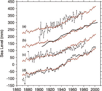
Figure ii.1 Global ocean-level time series from Church and White (2006; reddish) compared with independent global sea-level time serial from (a) Trupin and Wahr (1992), (b) Holgate (2007), (c) Gornitz and Lebedeff (1987), and (d) Jevrejeva et al. (2006) in black. Time series are arbitrarily shifted vertically for clarity. SOURCE: Woodworth et al. (2009).

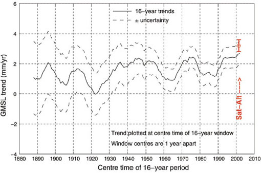
FIGURE two.2 Sixteen-year running averages of global body of water-level rising trends showing variability in rates over curt timescales. SOURCE: Church and White (2011).

Suggested Commendation:"2 Measured Global Sea-Level Rise." National Research Council. 2012. Sea-Level Rise for the Coasts of California, Oregon, and Washington: Past, Nowadays, and Future. Washington, DC: The National Academies Press. doi: 10.17226/13389.

×

Recent Estimates

Recent estimates of rates of global ocean-level rise are presented in Table 2.ane. In general, the new estimates over the unabridged 20th century are similar to those reported in the IPCC Quaternary Assessment Report. Rates for the last decade of the 20th century are college and similar to IPCC (2007) rates estimated from satellite altimetry and confirmed by tide gages (run across results of Jevrejeva et al., 2008; Merrifield et al., 2009; and Church and White, 2011). Because of natural temporal (due east.g., Effigy 2.2) and spatial variability in the sea-level signal, the meaning of the college rates of global body of water-level rising since the early 1990s is subject to interpretation. For example, Merrifield et al. (2009) attributed most of the contempo rise to higher rates of body of water-level ascent in the Southern Hemisphere and tropical regions, which had been seen past Cabanes et al. (2001) in satellite altimetry information.

It is likewise possible that the recent higher rate of sea-level rise represents an acceleration in the long-term trend. The record of sea-level ascent is punctuated by periods of dispatch and deceleration. Jevrejeva et al. (2008) used a Monte-Carlo-Singular Spectrum Analysis to remove the ii- to 30-year variability from more than i,000 tide gage records from around the world. They found an acceleration of 0.01 mm yr^-2 over the entire 300-twelvemonth period, with 60- to 65-yr periodicity in dispatch and deceleration for the preindustrial 18th and 19th centuries. The fastest rises in bounding main level occurred between 1920 and 1950 (upward to 2.5 mm yr^-ane) and between 1992 and 2002 (3.iv mm twelvemonth^-one; Jevrejeva et al., 2008). Many, but not all long tide gage records around the earth show an acceleration in global sea-level rise around 1920–1930 and a deceleration around 1960 (Woodworth et al., 2009; see besides Effigy 2.1). Although Houston and Dean (2011) plant a slight deceleration since 1930, Rahmstorf and Vermeer (2011) argued that this result reflects the pick of start date (1930) and the regional character of the gages used in their analysis.

Even if the college rates since the 1990s stand for a persistent acceleration in sea-level rise, pregnant additional acceleration would be required to attain usually projected sea levels (east.thousand., Hansen, 2007; Rahmstorf, 2007; Vermeer and Rahmstorf, 2009). For example, taking a charge per unit of 3.1 mm yr^-ane from satellite altimetry, bounding main level would rise only 0.28 m over the side by side 89 years. To reach one one thousand by 2100 would crave a positive acceleration of 0.182 mm yr^-2 for the entire time catamenia, based on the following quadratic equation:

H = H ₀ + (b × t) + (c/2) t²,

where H ₀ is the current ocean level, b is the linear charge per unit of sea-level rise, and c is the acceleration in units of mm yr^-2. In this example, dispatch would account for more 72 percent of the futurity sea-level rise. Such rapid acceleration is not seen in the 20th century tide gage record, except for short periods of fourth dimension, such as the 1930s and the 1990s (Effigy 2.2).

TABLE 2.1 Rates of Global Sea-Level Rising Estimated from Tide Gages

Source	Period	Sampling	Rate of Sea-Level Rise (mm twelvemonth-1)
IPCC(2007)	1900–2000	Not specified	1.7 ± 0.v
	1961–2003		1.8 ± 0.5
Church building and White (2006)	1870–1935	400 gages, global coverage	0.71 ± 0.4
	1956–2001		1.84 ± 0.19
Holgate (2007)	1904–1953	9 gages, by and large Northern Hemisphere	2.03 ± 0.35
	1904–2003		i.45 ± 0.34
	1904–2003		1.74 ± 0.16
Shum and Kuo (2011)	1900–2006	500 gages, global coverage	i.65 ± 0.4
Domingues et al. (2008)	1961–2003	Not specified	one.6 ± 0.two
Church and White (2011)	1900–2009	400 gages, global coverage	ane.seven ± 0.2
	1993–2009		2.8 ± 0.viii
Jevrejeva et al. (2008)	1992–2002	1,023 gages, global coverage	three.4
Merrifield et al. (2009)	1993–2007	134 gages, global coverage	3.2 ± 0.iv

Suggested Citation:"two Measured Global Body of water-Level Ascension." National Research Council. 2012. Sea-Level Ascension for the Coasts of California, Oregon, and Washington: Past, Nowadays, and Hereafter. Washington, DC: The National Academies Press. doi: 10.17226/13389.

×

SATELLITE ALTIMETRY

Satellite altimeters mensurate the body of water-surface height with respect to the Globe's middle of mass (Box ii.3). The satellite measurement also includes large-scale deformation of the bounding main basins caused past glacial isostatic adjustment (GIA), which must be removed from the indicate to obtain the ocean book alter. The global mean sea level is calculated by averaging measurements of sea-surface acme fabricated by the various altimeters, 3 of which are currently operating, which revisit a given spot on the Earth every 10 to 35 days.

Recent altimetry estimates of sea-level ascension are similar to those reported in the IPCC Fourth Assessment Report, ranging from 3.ii to three.3 mm yr^-1 from 1992 to 2010 (Table 2.2), and 2.ix ± 0.4 mm twelvemonth^-one from 1985 to 2010. The latter estimate includes data from higher latitudes and has a gap in data from 1988 to 1991 (Effigy ii.3). A recent assay of the full error budget due to musical instrument, orbit, media propagation errors, and geophysical corrections and their drifts suggests an uncertainty of ~0.4–0.5 mm twelvemonth^-i (Ablain et al., 2009), in agreement with external scale using information from island tide gages (Mitchum et al., 2010).

The regional variability in sea level seen in many tide cuff analyses has been confirmed by satellite altimetry records. Figure 2.4 shows the regional variation in sea-level trends in the global oceans based on 25 years (1985–2010 with a iii-yr data gap) of satellite altimetry data. The largest variations are in the western Pacific and eastern Indian oceans, where sea level has been ascent much faster than the global mean (warm colors in Figure ii.4). Bounding main level has been dropping in other areas, including the eastern Pacific Sea (cool colors in Effigy two.4). The IPCC concluded that these spatial patterns reflect interannual to interdecadal variability resulting from the El Niño-Southern Oscillation, the Northward Atlantic Oscillation, the Pacific Decadal Oscillation, and other climate patterns (Bindoff et al., 2007).

Satellite altimetry and tide gage estimates of sea-level change over the same timespan are in good agreement (e.g., Nerem et al., 2010). However, there are significant differences between long-term trends in tide gage records and the shorter satellite altimetry records. For case, Shum and Kuo (2011) estimated a tide-gage trend of 1.50 mm yr^-1 for 1880–2008 and a satellite altimetry tendency of ii.59 mm twelvemonth^-ane for 1985–1987 and 1991–2010 (Effigy two.5). Differences in trends for the two types of measurements for other data periods accept as well been reported (eastward.one thousand., Church and White, 2011). These differences are probable due to contamination of the altimetry trend by interannual or longer variations in the bounding main (e.g., Willis et al., 2010; Shum and Kuo, 2011) and, to a smaller extent, to sampling biases. Satellite altimetry records are shorter than tide gage records but cover more of the global ocean (81.5°N–81.v°S in Figure two.5). In improver, the body of water-level betoken from altimetry is dominated past the open ocean whereas the signal from tide gages is more strongly afflicted by the coastal ocean (e.k., Holgate and Woodworth, 2004).

GRAVITY RECOVERY AND CLIMATE EXPERIMENT (GRACE)

The GRACE mission makes detailed measurements of the Earth'due south gravity field and its variability over fourth dimension. Amidst the gravity variations detected by GRACE are mass changes in the ocean and land reservoirs (due east.k., country ice, groundwater) that contribute to sea-level change (Box 2.iv). The state ice and water components are discussed in Chapter 3. For the ocean component, GRACE measures the bounding main bottom pressure—the sum of the mass of the ocean and atmosphere above—at spatial resolutions of ~500 km. Sea bottom pressure changes when winds movement water beyond the ocean surface or when water is added to the oceans (e.g., through water ice melt, stream runoff), increasing the sea mass. The body of water mass change is determined by computing gravity field changes from the GRACE signal (Chambers et al., 2004; Tapley et al., 2004), and then correcting for the issue of glacial isostatic adjustment and high frequency ocean responses to wind and surface pressure forcing. When combined with other observations—such as altimetry data that have been corrected for temperature and salinity furnishings—GRACE data offer a potential ways of distinguishing how much global sea-level change is due to changes in mass and how much is due to changes in temperature and salinity.

Currently, however, there are difficulties associated with using GRACE data to infer bounding main mass changes. Changes in gravity over the sea, and thus the sea bottom pressure signal, are small relative to

Suggested Citation:"ii Measured Global Bounding main-Level Ascension." National Inquiry Council. 2012. Sea-Level Ascent for the Coasts of California, Oregon, and Washington: Past, Present, and Futurity. Washington, DC: The National Academies Printing. doi: ten.17226/13389.

×

BOX ii.3
Satellite Radar Altimetry Measurements

The start altimeter mission observing the global ocean was launched in 1978 (Seasat), just routine measurements of sea level from satellites began with the launch of TOPEX/Poseidon (1992–2006) and ERS-1 (1991–2000), and continued with ERS-ii (1996–2011), Geosat Follow-on (1998–2001), Jason-1 (2001–nowadays), Envisat (2002–present), Jason-2 (2008–present), and Cryosat-two (2010–present). Although these satellites are sometimes maneuvered in geodetic phases or interleave orbits, they accept occupied essentially the same ground tracks equally 10-twenty-four hour period, 17-day, or 35-day repeat orbits, providing a long data prepare of compatible observations. These satellites were equipped with radar altimeters to decide the distance between the satellite and the sea surface (see Figure). The location of the satellite, which has to be accurately known at all times, is adamant using tracking data from the Satellite Laser Ranging network, the Doppler Orbitography and Radio-positioning Integrated by Satellite (DORIS) country-based beacons, and the Global Navigation Satellite System (GNSS). Using the range or range-rate information from these tracking systems, the position and velocity of the satellite are determined and the radial orbit is and so calculated. The sea surface is estimated by averaging measurements taken over a 10-, 17-, or 35-day satellite track repeat bicycle. The accurateness of the sea surface acme measurements for TOPEX-form altimetry systems, considered to be the near authentic among the radar altimetry missions due to their optimal orbital sampling and high musical instrument precision, is a few cm (1 σ), afterwards correcting for instrument and media errors and geophysical phenomena.

The TOPEX and Jason satellites measure(d) the global ocean to latitudes of 66° north and south. Satellite altimeters that extend observations into the polar ocean include Geosat (1984–1987) and Geosat Follow-on, which covered latitudes of 71° north and south; ERS-1 and -ii and Envisat, which cover latitudes of 81.5° north and s; and Cryosat-2, which covers latitudes of 88° due north and southward. Their repeat orbits are longer than the TOPEX and Jason satellites: 17 days for Geosat and Geosat Follow-on, 35 days for ERS-i and -2 and Envisat, and 365 days with xxx-day subcycles for Cryosat-two.

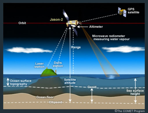
FIGURE The Jason-2 satellite uses a radar altimetry musical instrument to accurately measure out sea-surface heights. SOURCE: COMET^® Website at <http://meted.ucar.edu/> of the University Corporation for Atmospheric Research, sponsored in part through cooperative understanding(southward) with the National Oceanic and Atmospheric Assistants, U.S. Department of Commerce. ©1997-2011 University Corporation for Atmospheric Research. All rights reserved.

Suggested Citation:"2 Measured Global Sea-Level Rise." National Inquiry Council. 2012. Sea-Level Rise for the Coasts of California, Oregon, and Washington: Past, Present, and Hereafter. Washington, DC: The National Academies Press. doi: 10.17226/13389.

×

TABLE 2.2 Rates of Global Body of water-Level Rise Estimated from Satellite Altimetry

Source	Period	Breadth	Instruments	Rate of Sea-Level Rise (mm yr-1) a
D. Chambers (personal advice)	1992–2010	± 66°	TOPEX and Jason-1, -2	3.3 ± 0.5
Nerem et al. (2010)	1992–2010	± 66°	TOPEX and Jason-i, -2	3.3 ± 0.v
Leuliette and Miller (2009)	1992–2010	± 66°	TOPEX and Jason-1, -2	three.ii ± 0.iii
Cazenave et al. (2009)	1992–2010	± 66°	TOPEX and Jason-one, -2	iii.3 ± 0.ii
Church building and White (2011)	1993–2009	± 66°	TOPEX and Jason-1, -2	three.ii ± 0.4
Shum and Kuo (2011)	1985–2010	± 81.five°	Geosat, Geosat Follow-on, ERS, TOPEX, Envisat, and Jason-1, -two	2.9 ± 0.5

^a All rates were corrected for glacial isostatic aligning using the ICE-5G (VM2) model (Peltier, 2004) and atmospheric force per unit area effects (meet Appendix B).

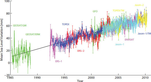
FIGURE 2.three Global ocean-level rise trends from dissimilar satellite altimeters for 1985–2010. The measured trend is ii.half-dozen ± 0.four mm year^-one, and the tendency corrected for glacial isostatic adjustment and atmospheric effects is 2.9 ± 0.4 mm yr^-one. Seasonal variations in the time series were non removed, but the trend was estimated simultaneously with periodicities associated with seasonal variations. SOURCE: Updated from Shum and Kuo (2011).

the GRACE accuracy limit and to the country gravity signal. Moreover, uncertainties in GIA models strongly impact the bounding main mass calculated from GRACE (e.g., Cazenave et al., 2009). Finally, GRACE data must be adapted to reduce loftier-frequency barotropic signals over the bounding main and over land (Flechtner, 2007) and to business relationship for motion of the geocenter (east.g., using laser ranging or Global Positioning Organization [GPS] information; Swenson et al., 2008). Once a consensus is reached on how to handle the processing and corrections, GRACE data may provide a valuable constraint on the ocean mass component of bounding main level and on the total sea-level upkeep.

CONCLUSIONS

Recent estimates of global body of water-level rising are in close understanding with estimates in the IPCC Quaternary Appraise-

Suggested Citation:"ii Measured Global Sea-Level Rising." National Research Council. 2012. Sea-Level Rise for the Coasts of California, Oregon, and Washington: By, Present, and Future. Washington, DC: The National Academies Press. doi: x.17226/13389.

×

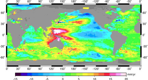
Effigy ii.four Regional variations in global sea-level ascension based on observations from satellite altimetry from 1985 to 2010. The data were corrected for glacial isostatic adjustment, atmospheric barotropic pressure response, and various instrument, media, and geophysical furnishings. SOURCE: Updated from Shum and Kuo (2011).

Figure two.five Comparison of ocean-level time series from tide gages (1880–2008; blue lines) and from satellite altimetry (1985–1987 and 1991–2010; red lines) later corrections for atmospheric barotropic pressure furnishings and glacial isostatic adjustment (using the ICE-5G [VM2] model, Peltier, 2004). The thin blueish line represents average monthly body of water level from global tide cuff data. The thick blueish line represents yearly sea-level changes from a moving average of tide gage observations, and the shaded area represents the ocean-level uncertainty, which reflects the number of gage sites used in the global averages, the number of data points, and the standard deviations of the fit of seasonal signals and the tendency of the original gage fourth dimension series. The thick red line is the yearly averaged altimetry body of water-level information. SOURCE: Updated from Shum and Kuo (2011).

Suggested Commendation:"2 Measured Global Sea-Level Rise." National Inquiry Council. 2012. Sea-Level Rise for the Coasts of California, Oregon, and Washington: Past, Present, and Hereafter. Washington, DC: The National Academies Printing. doi: 10.17226/13389.

×

BOX 2.4
GRACE Measurements

The Gravity Recovery and Climate Experiment measures changes of the mass distribution on Globe. The twin satellites travel in the same polar orbit 500 km above the Earth, with one satellite leading the other by approximately 220 km (Figure). When the lead satellite passes over a region of relatively high mass, it volition accelerate considering of increased gravitational allure and will increment the distance betwixt the satellites. On the other side of the region of high mass, it will boring again. The same effect applies to the trailing satellite. Past monitoring the irresolute distances between the satellites, and knowing their positions in space accurately via GPS and star cameras, the distribution of mass below the satellites can exist determined. Mass redistributions of the Earth are manifested in temporal gravity signals with a monthly sampling and spatial resolution longer than 300–400 km (half-wavelength; Tapley et al., 2004). GRACE information can be used to mensurate changes in mass of the ocean and its land reservoirs (due east.thou., country ice and groundwater; meet Chapter 3). Launched in 2002, the mission is expected to end in 2015.

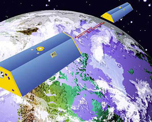
Effigy An artist's concept of GRACE satellites with ranging link between the two arts and crafts. SOURCE: National Helmsmanship and Space Administration.

ment Report, with long-term (50–100 years) rates of about one.8 mm yr^-i estimated from tide gages, and recent (mail service-1990) rates of about iii.2 mm yr^-1 estimated from satellite altimetry and tide gages. The higher rates of recent body of water-level rise may reflect interannual and longer variations due to ENSO and other climate patterns. Increases of iii–four times the current rate would be required to realize scenarios of i m sea-level rise by 2100. Such an acceleration has not yet been detected.

parrishwought.blogspot.com

Source: https://www.nap.edu/read/13389/chapter/4

Share this post